"""
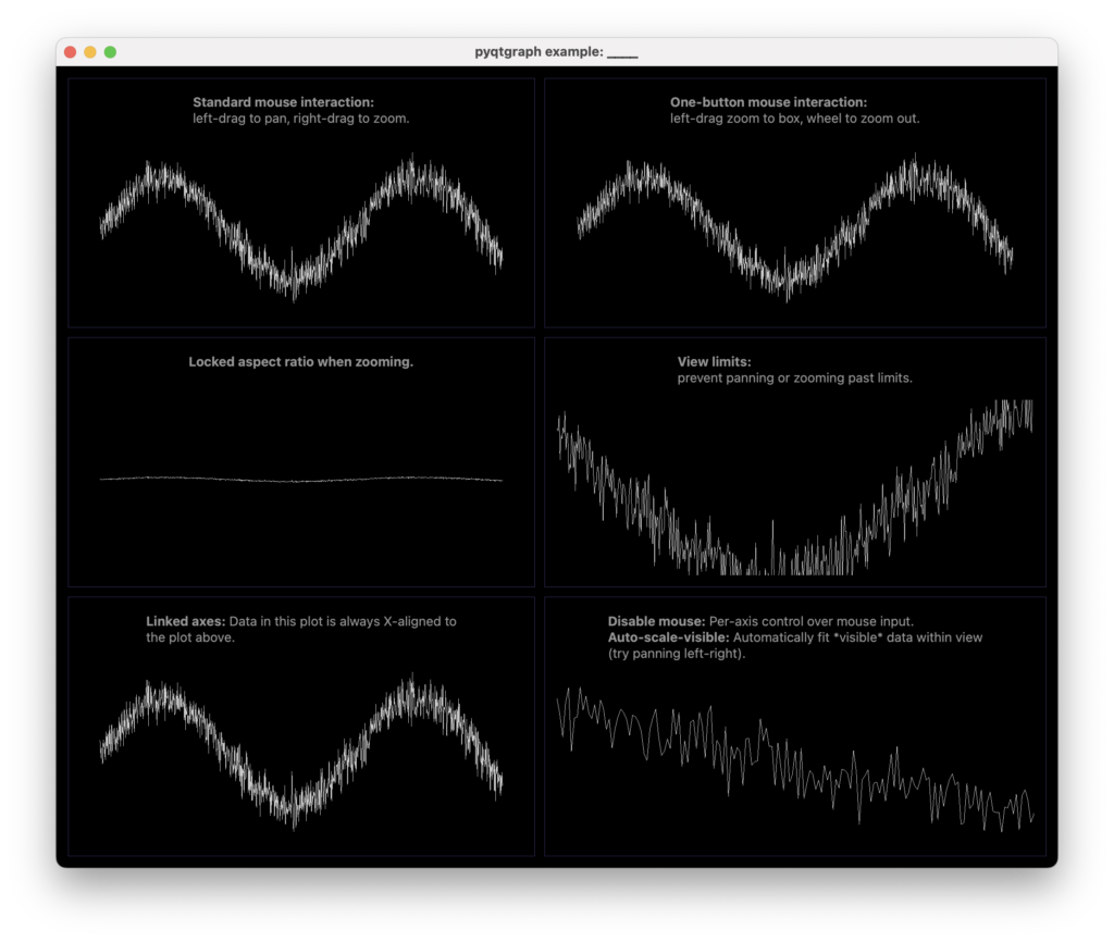
ViewBox is the general-purpose graphical container that allows the user to
zoom / pan to inspect any area of a 2D coordinate system.
This example demonstrates many of the features ViewBox provides.
"""
import numpy as np
import pyqtgraph as pg
x = np.arange(1000, dtype=float)
y = np.random.normal(size=1000)
y += 5 * np.sin(x/100)
win = pg.GraphicsLayoutWidget(show=True)
win.setWindowTitle('pyqtgraph example: ____')
win.resize(1000, 800)
win.ci.setBorder((50, 50, 100))
sub1 = win.addLayout()
sub1.addLabel("<b>Standard mouse interaction:</b><br>left-drag to pan, right-drag to zoom.")
sub1.nextRow()
v1 = sub1.addViewBox()
l1 = pg.PlotDataItem(y)
v1.addItem(l1)
sub2 = win.addLayout()
sub2.addLabel("<b>One-button mouse interaction:</b><br>left-drag zoom to box, wheel to zoom out.")
sub2.nextRow()
v2 = sub2.addViewBox()
v2.setMouseMode(v2.RectMode)
l2 = pg.PlotDataItem(y)
v2.addItem(l2)
win.nextRow()
sub3 = win.addLayout()
sub3.addLabel("<b>Locked aspect ratio when zooming.</b>")
sub3.nextRow()
v3 = sub3.addViewBox()
v3.setAspectLocked(1.0)
l3 = pg.PlotDataItem(y)
v3.addItem(l3)
sub4 = win.addLayout()
sub4.addLabel("<b>View limits:</b><br>prevent panning or zooming past limits.")
sub4.nextRow()
v4 = sub4.addViewBox()
v4.setLimits(xMin=-100, xMax=1100,
minXRange=20, maxXRange=500,
yMin=-10, yMax=10,
minYRange=1, maxYRange=10)
l4 = pg.PlotDataItem(y)
v4.addItem(l4)
win.nextRow()
sub5 = win.addLayout()
sub5.addLabel("<b>Linked axes:</b> Data in this plot is always X-aligned to<br>the plot above.")
sub5.nextRow()
v5 = sub5.addViewBox()
v5.setXLink(v3)
l5 = pg.PlotDataItem(y)
v5.addItem(l5)
sub6 = win.addLayout()
sub6.addLabel("<b>Disable mouse:</b> Per-axis control over mouse input.<br>"
"<b>Auto-scale-visible:</b> Automatically fit *visible* data within view<br>"
"(try panning left-right).")
sub6.nextRow()
v6 = sub6.addViewBox()
v6.setMouseEnabled(x=True, y=False)
v6.enableAutoRange(x=False, y=True)
v6.setXRange(300, 450)
v6.setAutoVisible(x=False, y=True)
l6 = pg.PlotDataItem(y)
v6.addItem(l6)
if __name__ == '__main__':
pg.exec()
Dock widgets
"""
This example demonstrates the use of pyqtgraph's dock widget system.

The dockarea system allows the design of user interfaces which can be rearranged by
the user at runtime. Docks can be moved, resized, stacked, and torn out of the main
window. This is similar in principle to the docking system built into Qt, but
offers a more deterministic dock placement API (in Qt it is very difficult to
programatically generate complex dock arrangements). Additionally, Qt's docks are
designed to be used as small panels around the outer edge of a window. Pyqtgraph's
docks were created with the notion that the entire window (or any portion of it)
would consist of dockable components.
"""

import numpy as np

import pyqtgraph as pg
from pyqtgraph.console import ConsoleWidget
from pyqtgraph.dockarea.Dock import Dock
from pyqtgraph.dockarea.DockArea import DockArea
from pyqtgraph.Qt import QtWidgets

app = pg.mkQApp("DockArea Example")
win = QtWidgets.QMainWindow()
area = DockArea()
win.setCentralWidget(area)
win.resize(1000,500)
win.setWindowTitle('pyqtgraph example: dockarea')

## Create docks, place them into the window one at a time.
## Note that size arguments are only a suggestion; docks will still have to
## fill the entire dock area and obey the limits of their internal widgets.
d1 = Dock("Dock1", size=(1, 1))     ## give this dock the minimum possible size
d2 = Dock("Dock2 - Console", size=(500,300), closable=True)
d3 = Dock("Dock3", size=(500,400))
d4 = Dock("Dock4 (tabbed) - Plot", size=(500,200))
d5 = Dock("Dock5 - Image", size=(500,200))
d6 = Dock("Dock6 (tabbed) - Plot", size=(500,200))
area.addDock(d1, 'left')      ## place d1 at left edge of dock area (it will fill the whole space since there are no other docks yet)
area.addDock(d2, 'right')     ## place d2 at right edge of dock area
area.addDock(d3, 'bottom', d1)## place d3 at bottom edge of d1
area.addDock(d4, 'right')     ## place d4 at right edge of dock area
area.addDock(d5, 'left', d1)  ## place d5 at left edge of d1
area.addDock(d6, 'top', d4)   ## place d5 at top edge of d4

## Test ability to move docks programatically after they have been placed
area.moveDock(d4, 'top', d2)     ## move d4 to top edge of d2
area.moveDock(d6, 'above', d4)   ## move d6 to stack on top of d4
area.moveDock(d5, 'top', d2)     ## move d5 to top edge of d2


## Add widgets into each dock

## first dock gets save/restore buttons
w1 = pg.LayoutWidget()
label = QtWidgets.QLabel(""" -- DockArea Example --
This window has 6 Dock widgets in it. Each dock can be dragged
by its title bar to occupy a different space within the window
but note that one dock has its title bar hidden). Additionally,
the borders between docks may be dragged to resize. Docks that are dragged on top
of one another are stacked in a tabbed layout. Double-click a dock title
bar to place it in its own window.
""")
saveBtn = QtWidgets.QPushButton('Save dock state')
restoreBtn = QtWidgets.QPushButton('Restore dock state')
restoreBtn.setEnabled(False)
w1.addWidget(label, row=0, col=0)
w1.addWidget(saveBtn, row=1, col=0)
w1.addWidget(restoreBtn, row=2, col=0)
d1.addWidget(w1)
state = None
def save():
    global state
    state = area.saveState()
    restoreBtn.setEnabled(True)
def load():
    global state
    area.restoreState(state)
saveBtn.clicked.connect(save)
restoreBtn.clicked.connect(load)


w2 = ConsoleWidget()
d2.addWidget(w2)

## Hide title bar on dock 3
d3.hideTitleBar()
w3 = pg.PlotWidget(title="Plot inside dock with no title bar")
w3.plot(np.random.normal(size=100))
d3.addWidget(w3)

w4 = pg.PlotWidget(title="Dock 4 plot")
w4.plot(np.random.normal(size=100))
d4.addWidget(w4)

w5 = pg.ImageView()
w5.setImage(np.random.normal(size=(100,100)))
d5.addWidget(w5)

w6 = pg.PlotWidget(title="Dock 6 plot")
w6.plot(np.random.normal(size=100))
d6.addWidget(w6)


win.show()


if __name__ == '__main__':
    pg.exec()
Console
"""
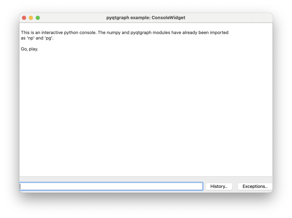
ConsoleWidget is used to allow execution of user-supplied python commands
in an application. It also includes a command history and functionality for trapping
and inspecting stack traces.
"""
import numpy as np
import pyqtgraph as pg
import pyqtgraph.console
app = pg.mkQApp()
## build an initial namespace for console commands to be executed in (this is optional;
## the user can always import these modules manually)
namespace = {'pg': pg, 'np': np}
## initial text to display in the console
text = """
This is an interactive python console. The numpy and pyqtgraph modules have already been imported
as 'np' and 'pg'.
Go, play.
"""
c = pyqtgraph.console.ConsoleWidget(namespace=namespace, text=text)
c.show()
c.setWindowTitle('pyqtgraph example: ConsoleWidget')
if __name__ == '__main__':
pg.exec()
Histgrams
"""
In this example we draw two different kinds of histogram.
"""

import numpy as np

import pyqtgraph as pg

win = pg.GraphicsLayoutWidget(show=True)
win.resize(800,350)
win.setWindowTitle('pyqtgraph example: Histogram')
plt1 = win.addPlot()
plt2 = win.addPlot()

## make interesting distribution of values
vals = np.hstack([np.random.normal(size=500), np.random.normal(size=260, loc=4)])

## compute standard histogram
y,x = np.histogram(vals, bins=np.linspace(-3, 8, 40))

## Using stepMode="center" causes the plot to draw two lines for each sample.
## notice that len(x) == len(y)+1
plt1.plot(x, y, stepMode="center", fillLevel=0, fillOutline=True, brush=(0,0,255,150))

## Now draw all points as a nicely-spaced scatter plot
y = pg.pseudoScatter(vals, spacing=0.15)
#plt2.plot(vals, y, pen=None, symbol='o', symbolSize=5)
plt2.plot(vals, y, pen=None, symbol='o', symbolSize=5, symbolPen=(255,255,255,200), symbolBrush=(0,0,255,150))

if __name__ == '__main__':
    pg.exec()
Beeswarm plot
"""
Example beeswarm / bar chart
"""

import numpy as np

import pyqtgraph as pg

win = pg.plot()
win.setWindowTitle('pyqtgraph example: beeswarm')

data = np.random.normal(size=(4,20))
data[0] += 5
data[1] += 7
data[2] += 5
data[3] = 10 + data[3] * 2

## Make bar graph
#bar = pg.BarGraphItem(x=range(4), height=data.mean(axis=1), width=0.5, brush=0.4)
#win.addItem(bar)

## add scatter plots on top
for i in range(4):
    xvals = pg.pseudoScatter(data[i], spacing=0.4, bidir=True) * 0.2
    win.plot(x=xvals+i, y=data[i], pen=None, symbol='o', symbolBrush=pg.intColor(i,6,maxValue=128))

## Make error bars
err = pg.ErrorBarItem(x=np.arange(4), y=data.mean(axis=1), height=data.std(axis=1), beam=0.5, pen={'color':'w', 'width':2})
win.addItem(err)


if __name__ == '__main__':
    pg.exec()
"""
This example demonstrates the different auto-ranging capabilities of ViewBoxes
"""

import time

import numpy as np

import pyqtgraph as pg
from pyqtgraph.Qt import QtCore

app = pg.mkQApp("Plot Auto Range Example")

win = pg.GraphicsLayoutWidget(show=True, title="Plot auto-range examples")
win.resize(800,600)
win.setWindowTitle('pyqtgraph example: PlotAutoRange')

d = np.random.normal(size=100)
d[50:54] += 10
p1 = win.addPlot(title="95th percentile range", y=d)
p1.enableAutoRange('y', 0.95)


p2 = win.addPlot(title="Auto Pan Only")
p2.setAutoPan(y=True)
curve = p2.plot()
t0 = time.time()

def update():
    t = time.time() - t0

    data = np.ones(100) * np.sin(t)
    data[50:60] += np.sin(t)
    curve.setData(data)

timer = QtCore.QTimer()
timer.timeout.connect(update)
timer.start(50)

if __name__ == '__main__':
    pg.exec()
Remote Plotting
"""
This example demonstrates the use of RemoteGraphicsView to improve performance in
applications with heavy load. It works by starting a second process to handle
all graphics rendering, thus freeing up the main process to do its work.

In this example, the update() function is very expensive and is called frequently.
After update() generates a new set of data, it can either plot directly to a local
plot (bottom) or remotely via a RemoteGraphicsView (top), allowing speed comparison
between the two cases. IF you have a multi-core CPU, it should be obvious that the
remote case is much faster.
"""

from time import perf_counter

import numpy as np

import pyqtgraph as pg
from pyqtgraph.Qt import QtCore, QtWidgets

app = pg.mkQApp()

view = pg.widgets.RemoteGraphicsView.RemoteGraphicsView()
pg.setConfigOptions(antialias=True)  ## this will be expensive for the local plot
view.pg.setConfigOptions(antialias=True)  ## prettier plots at no cost to the main process!
view.setWindowTitle('pyqtgraph example: RemoteSpeedTest')

app.aboutToQuit.connect(view.close)

label = QtWidgets.QLabel()
rcheck = QtWidgets.QCheckBox('plot remote')
rcheck.setChecked(True)
lcheck = QtWidgets.QCheckBox('plot local')
lplt = pg.PlotWidget()
layout = pg.LayoutWidget()
layout.addWidget(rcheck)
layout.addWidget(lcheck)
layout.addWidget(label)
layout.addWidget(view, row=1, col=0, colspan=3)
layout.addWidget(lplt, row=2, col=0, colspan=3)
layout.resize(800,800)
layout.show()

## Create a PlotItem in the remote process that will be displayed locally
rplt = view.pg.PlotItem()
rplt._setProxyOptions(deferGetattr=True)  ## speeds up access to rplt.plot
view.setCentralItem(rplt)

lastUpdate = perf_counter()
avgFps = 0.0

def update():
    global check, label, plt, lastUpdate, avgFps, rpltfunc
    data = np.random.normal(size=(10000,50)).sum(axis=1)
    data += 5 * np.sin(np.linspace(0, 10, data.shape[0]))

    if rcheck.isChecked():
        rplt.plot(data, clear=True, _callSync='off')  ## We do not expect a return value.
                                                      ## By turning off callSync, we tell
                                                      ## the proxy that it does not need to
                                                      ## wait for a reply from the remote
                                                      ## process.
    if lcheck.isChecked():
        lplt.plot(data, clear=True)

    now = perf_counter()
    fps = 1.0 / (now - lastUpdate)
    lastUpdate = now
    avgFps = avgFps * 0.8 + fps * 0.2
    label.setText("Generating %0.2f fps" % avgFps)

timer = QtCore.QTimer()
timer.timeout.connect(update)
timer.start(0)

if __name__ == '__main__':
    pg.exec()
Scrolling plots
"""
Various methods of drawing scrolling plots.
"""

from time import perf_counter

import numpy as np

import pyqtgraph as pg

win = pg.GraphicsLayoutWidget(show=True)
win.setWindowTitle('pyqtgraph example: Scrolling Plots')


# 1) Simplest approach -- update data in the array such that plot appears to scroll
#    In these examples, the array size is fixed.
p1 = win.addPlot()
p2 = win.addPlot()
data1 = np.random.normal(size=300)
curve1 = p1.plot(data1)
curve2 = p2.plot(data1)
ptr1 = 0
def update1():
    global data1, ptr1
    data1[:-1] = data1[1:]  # shift data in the array one sample left
                            # (see also: np.roll)
    data1[-1] = np.random.normal()
    curve1.setData(data1)

    ptr1 += 1
    curve2.setData(data1)
    curve2.setPos(ptr1, 0)


# 2) Allow data to accumulate. In these examples, the array doubles in length
#    whenever it is full.
win.nextRow()
p3 = win.addPlot()
p4 = win.addPlot()
# Use automatic downsampling and clipping to reduce the drawing load
p3.setDownsampling(mode='peak')
p4.setDownsampling(mode='peak')
p3.setClipToView(True)
p4.setClipToView(True)
p3.setRange(xRange=[-100, 0])
p3.setLimits(xMax=0)
curve3 = p3.plot()
curve4 = p4.plot()

data3 = np.empty(100)
ptr3 = 0

def update2():
    global data3, ptr3
    data3[ptr3] = np.random.normal()
    ptr3 += 1
    if ptr3 >= data3.shape[0]:
        tmp = data3
        data3 = np.empty(data3.shape[0] * 2)
        data3[:tmp.shape[0]] = tmp
    curve3.setData(data3[:ptr3])
    curve3.setPos(-ptr3, 0)
    curve4.setData(data3[:ptr3])


# 3) Plot in chunks, adding one new plot curve for every 100 samples
chunkSize = 100
# Remove chunks after we have 10
maxChunks = 10
startTime = perf_counter()
win.nextRow()
p5 = win.addPlot(colspan=2)
p5.setLabel('bottom', 'Time', 's')
p5.setXRange(-10, 0)
curves = []
data5 = np.empty((chunkSize+1,2))
ptr5 = 0

def update3():
    global p5, data5, ptr5, curves
    now = perf_counter()
    for c in curves:
        c.setPos(-(now-startTime), 0)

    i = ptr5 % chunkSize
    if i == 0:
        curve = p5.plot()
        curves.append(curve)
        last = data5[-1]
        data5 = np.empty((chunkSize+1,2))
        data5[0] = last
        while len(curves) > maxChunks:
            c = curves.pop(0)
            p5.removeItem(c)
    else:
        curve = curves[-1]
    data5[i+1,0] = now - startTime
    data5[i+1,1] = np.random.normal()
    curve.setData(x=data5[:i+2, 0], y=data5[:i+2, 1])
    ptr5 += 1


# update all plots
def update():
    update1()
    update2()
    update3()
timer = pg.QtCore.QTimer()
timer.timeout.connect(update)
timer.start(50)

if __name__ == '__main__':
    pg.exec()
HDF5 big data
"""
In this example we create a subclass of PlotCurveItem for displaying a very large
data set from an HDF5 file that does not fit in memory.

The basic approach is to override PlotCurveItem.viewRangeChanged such that it
reads only the portion of the HDF5 data that is necessary to display the visible
portion of the data. This is further downsampled to reduce the number of samples
being displayed.

A more clever implementation of this class would employ some kind of caching
to avoid re-reading the entire visible waveform at every update.
"""

import os
import sys

import h5py
import numpy as np

import pyqtgraph as pg
from pyqtgraph.Qt import QtWidgets

pg.mkQApp()


plt = pg.plot()
plt.setWindowTitle('pyqtgraph example: HDF5 big data')
plt.enableAutoRange(False, False)
plt.setXRange(0, 500)

class HDF5Plot(pg.PlotCurveItem):
    def __init__(self, *args, **kwds):
        self.hdf5 = None
        self.limit = 10000 # maximum number of samples to be plotted
        pg.PlotCurveItem.__init__(self, *args, **kwds)

    def setHDF5(self, data):
        self.hdf5 = data
        self.updateHDF5Plot()

    def viewRangeChanged(self):
        self.updateHDF5Plot()

    def updateHDF5Plot(self):
        if self.hdf5 is None:
            self.setData([])
            return

        vb = self.getViewBox()
        if vb is None:
            return  # no ViewBox yet

        # Determine what data range must be read from HDF5
        range_ = vb.viewRange()[0]
        start = max(0,int(range_[0])-1)
        stop = min(len(self.hdf5), int(range_[1]+2))

        # Decide by how much we should downsample
        ds = int((stop-start) / self.limit) + 1

        if ds == 1:
            # Small enough to display with no intervention.
            visible = self.hdf5[start:stop]
            scale = 1
        else:
            # Here convert data into a down-sampled array suitable for visualizing.
            # Must do this piecewise to limit memory usage.
            samples = 1 + ((stop-start) // ds)
            visible = np.zeros(samples*2, dtype=self.hdf5.dtype)
            sourcePtr = start
            targetPtr = 0

            # read data in chunks of ~1M samples
            chunkSize = (1000000//ds) * ds
            while sourcePtr < stop-1:
                chunk = self.hdf5[sourcePtr:min(stop,sourcePtr+chunkSize)]
                sourcePtr += len(chunk)

                # reshape chunk to be integral multiple of ds
                chunk = chunk[:(len(chunk)//ds) * ds].reshape(len(chunk)//ds, ds)

                # compute max and min
                chunkMax = chunk.max(axis=1)
                chunkMin = chunk.min(axis=1)

                # interleave min and max into plot data to preserve envelope shape
                visible[targetPtr:targetPtr+chunk.shape[0]*2:2] = chunkMin
                visible[1+targetPtr:1+targetPtr+chunk.shape[0]*2:2] = chunkMax
                targetPtr += chunk.shape[0]*2

            visible = visible[:targetPtr]
            scale = ds * 0.5

        self.setData(visible) # update the plot
        self.setPos(start, 0) # shift to match starting index
        self.resetTransform()
        self.scale(scale, 1)  # scale to match downsampling


def createFile(finalSize=2000000000):
    """Create a large HDF5 data file for testing.
    Data consists of 1M random samples tiled through the end of the array.
    """

    chunk = np.random.normal(size=1000000).astype(np.float32)

    f = h5py.File('test.hdf5', 'w')
    f.create_dataset('data', data=chunk, chunks=True, maxshape=(None,))
    data = f['data']

    nChunks = finalSize // (chunk.size * chunk.itemsize)
    with pg.ProgressDialog("Generating test.hdf5...", 0, nChunks) as dlg:
        for i in range(nChunks):
            newshape = [data.shape[0] + chunk.shape[0]]
            data.resize(newshape)
            data[-chunk.shape[0]:] = chunk
            dlg += 1
            if dlg.wasCanceled():
                f.close()
                os.remove('test.hdf5')
                sys.exit()
        dlg += 1
    f.close()

if len(sys.argv) > 1:
    fileName = sys.argv[1]
else:
    fileName = 'test.hdf5'
    if not os.path.isfile(fileName):
        size, ok = QtWidgets.QInputDialog.getDouble(None, "Create HDF5 Dataset?", "This demo requires a large HDF5 array. To generate a file, enter the array size (in GB) and press OK.", 2.0)
        if not ok:
            sys.exit(0)
        else:
            createFile(int(size*1e9))
        #raise Exception("No suitable HDF5 file found. Use createFile() to generate an example file.")

f = h5py.File(fileName, 'r')
curve = HDF5Plot()
curve.setHDF5(f['data'])
plt.addItem(curve)

if __name__ == '__main__':
    pg.exec()


コメント